Particle Swarm Optimization (PSO) Algorithm

Particle Swarm Optimization (PSO) is a popular metaheuristic method that mimics the collective migration of swarms of birds to find optimal solutions to complex problems. The most widely used algorithms in engineering, finance, and in biology is due to their ability to analyze and directly apply. The algorithm is highly advantageous due to its ability to quickly find a solution by re-adjusting the effect position This process considers the optimal position of each individual particle and the optimal position of the entire system as a whole.

Moreover, its significant level of parallelizability makes it highly suitable for implementation on modern computing systems, hence improving processing speeds and scalability.

The simplicity and efficacy of PSO are widely recognized qualities that contribute to its success. PSO requires fewer parameters to be fine-tuned in comparison to other metaheuristic algorithms such as genetic algorithms and simulated annealing. Implementing this approach is simplified and requires fewer time and computational resources. The algorithm's adeptness in managing non-linear, multi-dimensional optimization problems with great efficiency has resulted in its widespread application in several domains. PSO, or Particle Swarm Optimization, is utilized in engineering to optimize design parameters with the goal of enhancing performance and reducing costs. In the field of economics, mathematical modeling is used to analyze and resolve complex financial issues. Similarly, in biology, it is employed to comprehend and simulate natural phenomena.

The versatility and efficiency of PSO have gained substantial support and regular collaboration in the scientific community. It frequently enhances other optimization approaches, such as genetic algorithms and simulated annealing, by combining them to create hybrid models that utilize the advantages of each method. Hybrid algorithms, such as those that integrate particle swarm optimization (PSO) with genetic algorithms, leverage the global search powers of PSO and the fine-tuning abilities of genetic algorithms. PSO is frequently integrated with machine learning algorithms to enhance the precision and dependability of predictions. This feature enhances its utility across various research domains and contexts.

Although particle swarm optimization has its benefits, it also encounters specific problems. A significant critique of this approach is its inclination to prematurely converge, particularly in intricate landscapes with numerous local optima, resulting in unsatisfactory solutions. In order to address this problem, several adjustments and improvements have been suggested for the fundamental PSO algorithm, including the incorporation of inertia weights, constriction factors, and velocity clamping. PSO has a restriction in that its performance is substantially influenced by the right setup of its parameters, such as cognitive and social factors. Improper configuration of parameters can lead to either a decrease in the speed at which convergence occurs or instability in the search process.

Here, we present the implementation of the PSO and is compared to analytical methods. First, the PSO is detailed with its governing equations. Second, the optimization problem is defined. Third, the algorithm is detailed. Finally, an analytical solution is proposed to compare it to the solution obtained by the PSO.

To summarize, particle swarm optimization has demonstrated its efficacy and adaptability in addressing various optimization challenges. However, it is essential to acknowledge its limitations and possible drawbacks. To fully utilize the potential of PSO in their respective disciplines, researchers and practitioners can overcome these limitations by comprehending and addressing them.

The Theory

In this section we show the theory behind the PSO algorithm and also describes the implementation in MATLAB. A test function is used to validate the behavior of the algorithm.

PSO algorithms are a type of meta-heuristic algorithm inspired by the behavior of bird flocking or fish swarming. Edward and Kennedy proposed it in 1995. These algorithms are similar to the continuous genetic algorithms starting with a random population matrix, where the particle contains the information of the variables as the chromosomes in the GA. However, they have no evolutionary operator such as crossover or mutation.

Each particle moves with continuous values about the cost surface with a velocity \(v\). At each time-step, the particle updates its velocity \(v_{m,n}\) and its position \(p_{m,n}\) based on local and global best solutions, with \(m,n\) being respectively the population size and number of parameters. The swarm has a cognitive (or individual) and social parameter \(\kappa_1\) and \(\kappa_2\), respectively. We can express the model as equation \ref{eq:pso}.

\[ v^{t+1}_{m,n} = \mu v^{t}_{m,n} + \underbrace{\kappa_1 r_1 (\mathbf{p}_{m,n} - \mathbf{p}^{t}_{m,n})}_{\text{individual}} + \underbrace{\kappa_2 r_2 (\mathbf{g}^{t}_{m,n} - \mathbf{p}^{t}_{m,n})}_{\text{social}} \]

Where \(\mathbf{p}^{t+1}_{m,n} = \mathbf{p}^{t}_{m,n} + v^{t+1}_{m,n}\) is the position of the particle at \(t\), notably the local minima, and \(\mathbf{g}\) is the global minimum. The parameters \(r_{1}\) and \(r_{2}\) \(\in [0,1]\) are a uniform random value meaning that the individual is affected by its own values or those of the other particles. This can be likened to the tendency of sometimes being egocentric and disregarding others, or alternatively, simply going with the flow. Neither approach guarantees convergence. In this scenario, one particle might have discovered the global optimum, but its companions seemed more entertaining. The next iteration he will rethink its actions. As the birds have a mass, the literature considers a inertia parameter \(\mu\) causing the particle to discover other places after a fast descent. In our case, \(\mu\) decreases as the number of iterations reaches its maximum.

To visualize the previous equation, let's consider the figure below.

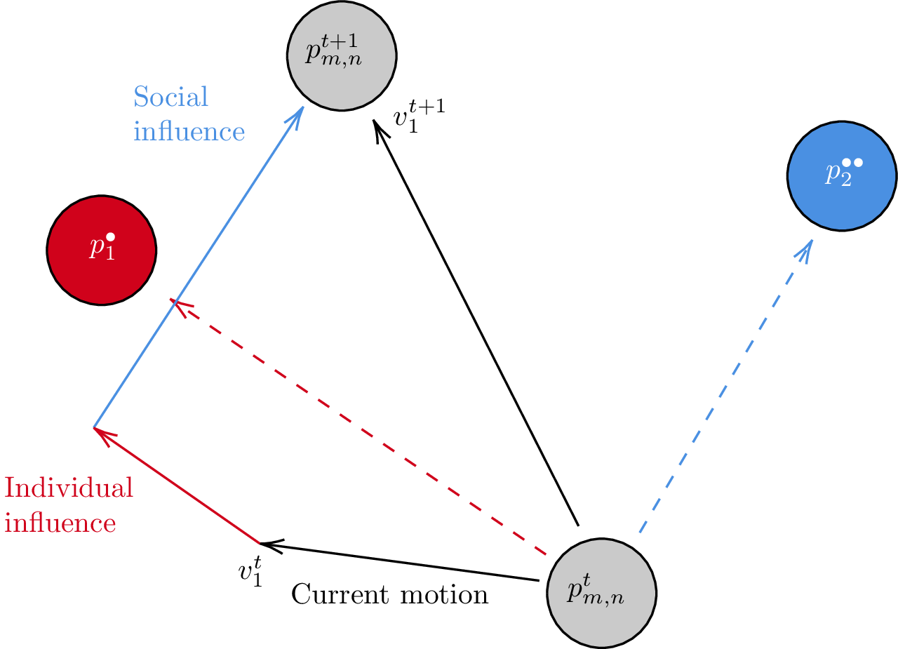
The particle \(p_{m,n}\) at a state \(t\) updates its position and velocity to a new state \(t+1\) with the information of its next individual information \(p^{\bullet}_1 = \mathbf{p}_1\) with some random weight \(r_1\) and the swarm global information \(p^{\bullet \bullet}_2 = \mathbf{g}\). Every particle does the same thing and, in that way, the social behavior emerges.

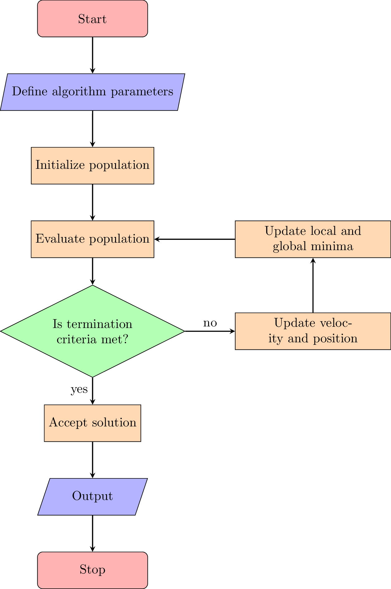
The algorithm starts with pre-defined parameters such as cognitive and social parameters, lower and upper bounds, number of variables in the problem, maximal iterations, ant the population size. Additionally and most importantly, the cost function is defined at this stage too. Once the algorithm is initialize, the population is evaluated with the cost function. Then, if a convergence criteria is met or the maximal number of iterations is achieved, the algorithm ends. If not, the velocity and position of each particle is updated and the local and global minima is calculated. See the figure below for illustration.

The optimization problem is shown in the following equation.

\[ \begin{aligned} \min \quad & f(\vec{X}) = (x_1 - 10)^2 + (x_2 - 20)^3 \\ \textrm{s.t.} \quad & g_1(\vec{X}) = -(x_{1}-5)^2-(x_{2}-5)^2+100 \leq 0 \\ & g_2(\vec{X}) = (x_{1}-6)^2+{x_2}-5)-82.81 \leq 0 \\ & 13 \geq x \geq 100 \\ & 0 \geq y \geq 100 \\ \end{aligned} \]

To transform the constrained problem into a unconstrained one, we make a transformation that defines a new objective function \(\mathcal{J}\) using the quadratic penalty function \(p_{i} \sum_{i} \max(0,g_{i})^{2}\), where \(p\) is an arbitrary scalar constant known as the penalty factor. The problem becomes equation:

\[ \mathcal{J}(\vec{X}) = f(\vec{X}) + p_{1} \max (0,g_{1}(\vec{X}))^{2} + p_{2} \max (0,g_{2}(\vec{X}))^{2}\ \]

This new objective function defines the search space (\(\mathcal{J} \in \mathbb{R}^2\)) of the particles to find the global minimum. In the next paragraph, we describe the algorithm. It takes as input the objective function \(f\), in the present case is equation \ref{eq:loss}, then the number of parameters \(n\), the lower and upper bounds \(\mathbf{lb}\) and \(\mathbf{ul}\) respectively, the maximum number of iterations \(T\), then the cognitive \(c_1\) and social \(c_2\) parameters, a constraint factor \(C\), and the population size \(m\).

\(\mathbf{X}\), \(\mathbf{V}\), \(\mathbf{P}\), \(\mathbf{g}\), \(\mathcal{J}\), and \(\mathcal{J}_p\) represent the positions, velocities, local best positions, global best position, costs, and local best costs respectively. \(\mathbf{r}_1\) and \(\mathbf{r}_2\) \(\in \mathbb{R}^{m \times n} \in [0,1]\) are random matrices. The velocity update equation includes the constriction factor \(C\) and inertia weight \(\mu\).

To summarize, this algorithm gives the global parameters \(\mathbf{g}\) and the evaluation of the cost function \(\mathcal{J}_p\).

Results

To solve this problem analytically, we use the lagrangian multipliers \(\lambda_1\) and \(\lambda_2\) for \(g_1\) and \(g_2\) respectively. This allow us to modify the objective function, or loss function \(\mathcal{L}\) into

\[ \mathcal{L}(\vec{X},\lambda_1,\lambda_2) = f(\vec{X}) + \lambda_{1} g_{1}(\vec{X}) + \lambda_{2} g_{2}(\vec{X}) \]

Then, to find the minimum of the new function, we set \(\nabla \mathcal{L} = 0\), so

\[ \nabla \mathcal{L} = \left( \frac{\partial \mathcal{L}}{\partial x_1}, \frac{\partial \mathcal{L}}{\partial x_2}, \frac{\partial \mathcal{L}}{\partial \lambda_1}, \frac{\partial \mathcal{L}}{\partial \lambda_2} \right) = 0. \]

Developing,

\[ \frac{\partial \mathcal{L}}{\partial x_{1}} = 3(x - 10)^2 + \lambda_{1} \left( -2(x - 5) \right) + \lambda_{2} \left( 2(x - 6) \right) \]

\[ \frac{\partial \mathcal{L}}{\partial x_{2}} = 3(y - 20)^2 + \lambda_{1} \left( -2(y - 5) \right) + \lambda_{2} \]

\[ \frac{\partial \mathcal{L}}{\partial \lambda_{1}} = -(x - 5)^2 - (y - 5)^2 + 100 \]

\[ \frac{\partial \mathcal{L}}{\partial \lambda_{2}} = (x - 6)^2 + (y - 5) - 82.81, \]

so for \(x_1 = 13.66\), \(x_2 = 0\), \(\lambda_1 = 2.32\), and \(\lambda_2 = 6.8658 \times 10^{-6}\), the solution of \(f(\vec{X}) = -7951\) is the solution \(\mathcal{L}\). To confirm that the solution is a minimum, the Laplacian \(\Delta \mathcal{L} > 0\), however the value being \(-98.0384\), meaning that the function is still decreasing at the solution point, but the problem is bounded. The given solution of the cost function is taken as reference.

On the other hand, the PSO algorithm gives an error of \(2,5154 \times 10^{-5}\) from the reference value, and the value of the variables at the solution being \(x_1 = 13.6663\), and \(x_2 = 0\), evaluating the cost function \(\mathcal{J} = -7950.8\). The time of execution is \(0.1535s\).

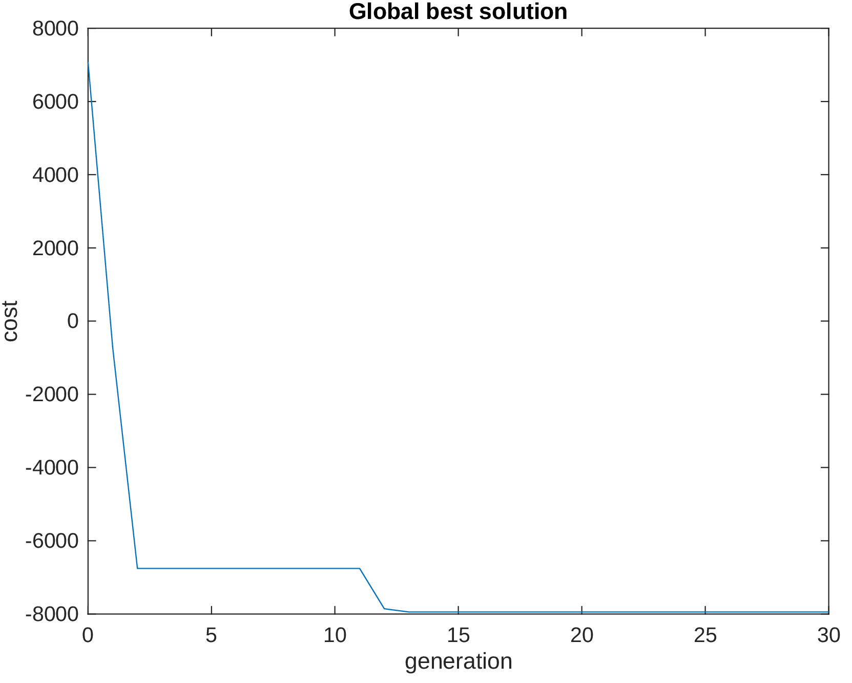
Here we show the evolution of the global minimum found by the algorithm at each iteration. We observe a rapid convergence towards the global minimum. The algorithm finds the solution after 16 iterations.

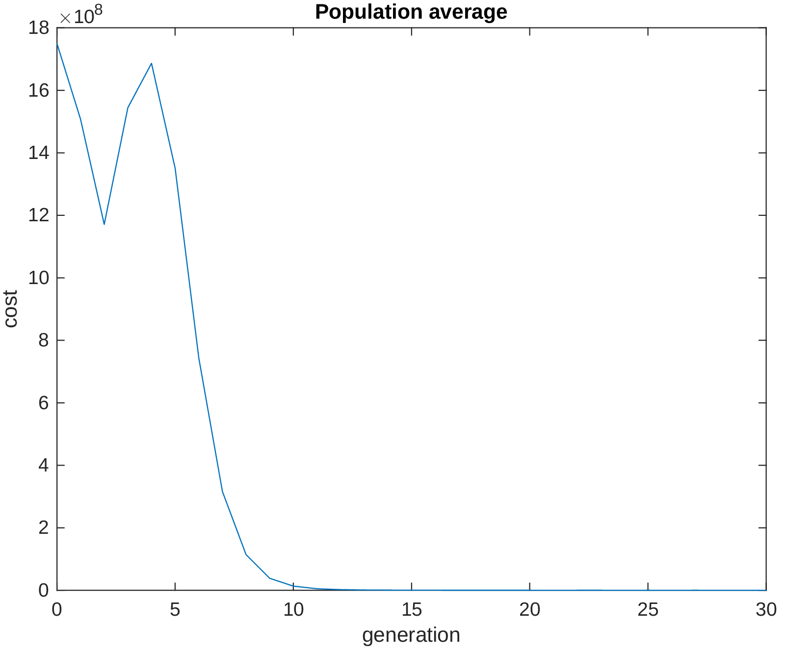
This figure shows the mean value of the whole population at time \(t \in [0,T]\). Similarly, it decreases as the population approaches the global minimum. However, the number is high as not all the particles reached the solution at the end of the iterations.

Finally, the next two figures show the evaluation of the constraint functions \(g_1\) and \(g_2\), respectively.

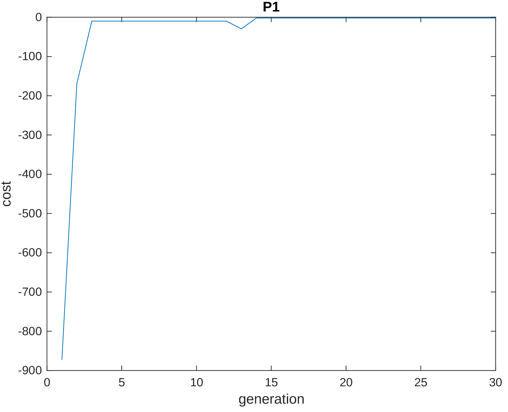
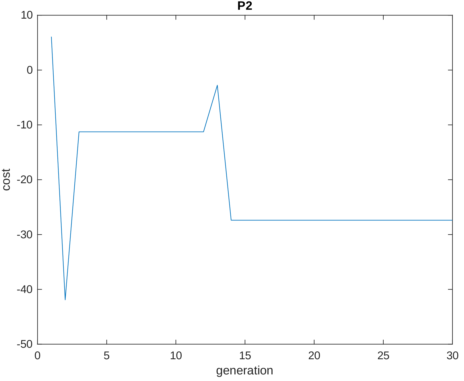
The results does not show the convergence rate. However, multiple runs were done and some times the algorithm ended up in a local solution.

Conclusions

The particle swarm optimization algorithm is capable of finding the global minimum of a multidimensional optimization problem with many local minima. The interaction between each particle creates a social behavior that finds the best solution. However, the parameters must be modified in order to solve the problem. The PSO allows to solve optimization problems that are not differentiable or discontinuous. In this work we evaluated the PSO with a test program that is bounded and with constraints. We showed the analytical solution and compared with the solution found numerically by the PSO.

The MATLAB Code

function [all_par,all_iter,minc] = parswarm(CostFunction,npar,lb,ub, ...
    maxit,cog,social,cnstr,popsize)
    ff = CostFunction; % Objective Function
    c1 = cog; % cognitive parameter
    c2 = social; % social parameter
    C  = cnstr; % constriction factor (inertia)
    varhi = ub; % uppber bound
    varlo = lb; % lower bound
    
    % Initializing swarm and velocities
    par = (varhi - varlo).*rand(popsize,npar) + varlo;
    vel = (varhi - varlo).*rand(popsize,npar) + varlo;
    
    % Evaluate initial population
    cost=feval(ff,par); % calculates population cost using ff
    costsize = size(cost);
    minc = zeros(maxit,costsize(2));
    meanc = zeros(maxit,costsize(2));
    minc(1,:) = min(cost);
    meanc(1,:) = mean(cost);
    globalmin=minc(1); % initialize global minimum
    
    % Initialize local minimum for each particle
    localpar = par; % location of local minima
    localcost = cost; % cost of local minima
    
    % Finding best particle in initial population
    [globalcost,indx] = min(cost);
    globalpar=par(indx,:);
    
    % Initialize arrays to store 'par' and 'iter'
    all_par = par(indx,:);
    all_iter = zeros(maxit, 1);
    
    %%%%%%%%%%%%%%%%%%%%%%%%%%%%%%%%%%%%%%%%%%%%%%%%%%%%%%%%
    % Start iterations
    iter = 0; % counter
    
    while iter < maxit
	iter = iter + 1;
	% update velocity = vel
	w=(maxit-iter)/maxit; %inertia weigth
	r1 = rand(popsize,npar); % random numbers
	r2 = rand(popsize,npar); % random numbers
	vel = C*(w*vel + c1 *r1.*(localpar-par) + ...
	    c2*r2.*(ones(popsize,1)*globalpar-par));
    
	% update particle positions
	par = par + vel; % updates particle position
	overlimit=par<=varhi; % bounds
	underlimit=par>=varlo;
	par=par.*overlimit+not(overlimit); % ensure p is within bounds
	par=par.*underlimit; %
    
	% Store 'par' and 'iter'
	all_par(iter,:) = globalpar;
	all_iter(iter) = iter;
	% Evaluate the new swarm
	cost = feval(ff,par); % evaluates cost of swarm
	% Updating the best local position for each particle
	bettercost = cost < localcost;
	localcost = localcost.*not(bettercost) + cost.*bettercost;
	localpar(bettercost,:) = par(bettercost,:);
	% Updating index g
	[temp, t] = min(localcost);
	if temp<globalcost
	    globalpar=par(t,:); indx=t; globalcost=temp;
	end
	% [iter globalpar globalcost] % print output each iteration
	minc(iter+1)=min(cost); % min for this iteration
	globalmin(iter+1)=globalcost; % best min so far
	meanc(iter+1)=mean(cost); % avg. cost for this iteration
    end % while
end % function

To test the code...

f = @(x) (x(:,1)-10).^3+(x(:,2)-20).^3;
P1 = @(x) -(x(:,1)-5).^2-(x(:,2)-5).^2+100;
P2 = @(x)  (x(:,1)-6).^2+(x(:,2)-5)-82.81;
lambda1 = 100;
lambda2 = 100;
C = @(x) f(x) + lambda1*max(0,P1(x)).^2 + lambda2*max(0,P2(x)).^2;
npar = 2; varhi = [100 100]; varlo = [13 0];
[par,iter,minc] = parswarm(C,npar,varlo,varhi,30,0.1,0.2,0.8,100);
p1 = feval(P1,par);
p2 = feval(P2,par);